

PermalinkIntroduction
Hello Reader, In this blog we'll be looking into the Internal working of Data Structure : HashTable,
HashTables are implemented in almost all the Object Oriented Programming Languages, like : Dictionaries in Python, Objects in JavaScript, ArrayLists in Java, Vectors in C++ etc.
we'll be implementing our own HashTables in Python, as Python is considered as one of the easy to read
language.
PermalinkPre-requisites
- Array
- LinkedList
- Basic Understanding of Big-O Notations
- Basics of Object Oriented Programming in Python
PermalinkImportance of Using HashTables
Hashtables plays a very important role in making programs run efficient and fast, the reason boils down to the running Time Complexities of hashtable , i.e
- O(1) - Inserting an Item
- O(1) - Deleting an Item
- O(1) - Searching an Item
let's look into the calculations.
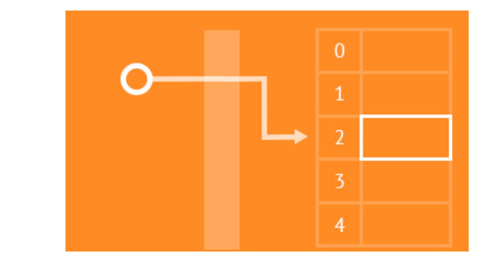
PermalinkStoring data in HashTable
We use Hashing strategy for storing data into a hashtable, In hashing we use Hash Functions , we pass the item that we need to store, in a hash function as a parameter to a function and the function in return gives us the hash code sometimes called as a hash message, after receiving the hash message we perform the message compression based on the bucket size of a table, we do it using a % operator on a hash code, so whatever gets returned from it acts as a index of an array and at that index we store the key along with the value, i.e key:value pair.
Basic hash function looks something like this code snippet below:
def hash_function(key,bucket_size):
    hash_value = hash(key)
    return hash_value % bucket_size
In this hash function we are using hash() function which is an inbuilt Python library function that returns the hash code and then we have used the modulo operator to get the index in the required bucket range. this returns us the index value where we will store the key:value pair.
time complexity of the inbuilt hash() is O(1) , so it's a constant time operation. Having such a functionality is good to have , but their are some certain challenges that comes when we try to hash the keys, i.e collisions in the indexes, their are chances to get the same index value for different keys causing collision in storing the data at that index, this all depends on the hash function we are using to index values accordingly.
A good hash function will not result in much collision of keys, which will later provides the required benefits of using hashtables by making the time complexities as expected.
let's discuss about the collision handling techniques
PermalinkHandling Collisions
Some of the approaches to handle collisions:
- Direct Chaining
- Linear Probing
- Quadratic Probing
The Inbuilt Libraries uses the the Direct Chaining approach sometimes as it makes the tables much efficient.
let's discuss about each one of them in detail:
Permalink- Direct Chaining:
In this approach, we store the head of the linkedlist on the index we got from the hash function, this way we'll be chaining the items in the form of the linkedlist, whenever the index of the different keys results in collision.
There are some limitations with the approach, if the hash function is not good then we'll end up getting all the keys forming a linkedlist in a single bucket which will then results in the performance issues.
So, for this problem, we have the universal hashing technique which gives us the uniform distribution of the keys, it uses the "group of hash functions" and then for each key the randomization algorithm choose the hash function in which the key get passed, this makes the distribution even better as compared to using only a single hash function.
Remember? , we have used the hash() inbuilt function, that function has already "universal hashing" implemented, so when we use it to generate the hash code, it provides the index accordingly.
we have something known as a Load Factor (⍺) , it describes the distribution of keys over buckets. The expression is defined as :
Load Factor (⍺) = N/B, N : number of keys, B: number of buckets
It describes the number of keys per bucket, the Load Factor (⍺) should be (≤ 0.7), for efficient search, insert, delete operations, if it goes beyond this value then we have to Rehash the keys, for rehashing we double the bucket capacity and then we perform insert operation for all the keys, this way the load factor remains under the required value.
The effective time complexity becomes,
- O(⍺) - Searching an Item
- O(⍺) - Inserting an Item
- O(⍺) - Deleting an Item
This makes the average case time complexity of O(1), in all 3 aspects because of universal hashing.
let's look into the implementation of direct chaining,
class Node:
  def __init__(self,key,value):
    self.key = key
    self.value = value
    self.next = None

class HashTable:
  def __init__(self,bucket_size):
    self.bucket_size = bucket_size
    self.hashtable = [None] * self.bucket_size
    self.total_keys = 0

  def insert(self,key,value):
    idx = hash(key) % self.bucket_size
    if not self.hashtable[idx]:
      self.hashtable[idx] = Node(key,value)
    else:
      temp = self.hashtable[idx]
      while temp.next != None:
        temp = temp.next
      temp.next = Node(key,value)
    self.total_keys += 1

  def search(self,key):
    idx = hash(key) % self.bucket_size
    if not self.hashtable[idx]:
      print(f"{key} Not found")
      return None
    else:
      temp = self.hashtable[idx]
      while temp != None:
        if temp.key == key:
          print(f"{key} found")
          return temp
        temp = temp.next
      print(f"{key} Not found")
      return None

  def delete(self,key):
    idx = hash(key) % self.bucket_size
    item_ref = self.search(key)
    if not item_ref:
      return f"{key} Not found"
    else:
      self.total_keys -= 1
      temp = self.hashtable[idx]
      if temp.key == item_ref.key:
        self.hashtable[idx] = temp.next
        return
      while temp != None:
        if temp.key == item_ref.key:
          break
        before_item = temp
        temp = temp.next
      before_item.next = item_ref.next


  def load_factor(self):
    return self.total_keys / self.bucket_size

  def rehashing(self):
    old_hashtable = self.hashtable
    self.bucket_size *= 2
    self.hashtable = [None] * self.bucket_size
    for head_ref in old_hashtable:
      temp = head_ref
      while temp != None:
        idx = hash(temp.key) % self.bucket_size
        if not self.hashtable[idx]:
          self.hashtable[idx] = Node(temp.key,temp.value)
        else:
          iter = self.hashtable[idx]
          while iter.next != None:
            iter = iter.next
          iter.next = Node(temp.key,temp.value)
        temp = temp.next

  def check_for_rehashing_requirement(self):
    if self.load_factor() > 0.7:
      return "Rehashing required"
    else:
      return "Rehashing not required"
Permalink- Linear Probing:
This approach is a part of Open Addressing, In this approach, we don't create a linkedlist like structure, rather we store a single key per bucket, so the number of keys == number of buckets , so whenever the collision takes place we linearly probe or linearly move one step at a time and find the next available slot/bucket where we can store the key:value pair, We have a probing function i.e,
index = hash(key) + P(x) where, P(x) = x, x ≥ 0
let's look into the implementation of Linear Probing,
class Node:
  def __init__(self,key,value):
    self.key = key
    self.value = value

class HashTable:
  def __init__(self,bucket_size):
    self.bucket_size = bucket_size
    self.hashtable = [None] * self.bucket_size

  def insert(self,key,value):
    idx = hash(key) % self.bucket_size
    i = 0
    while i < self.bucket_size:
      if not self.hashtable[idx]:
        self.hashtable[idx] = Node(key,value)
        return
      idx = (idx+1) % self.bucket_size
      i+=1
    print("No space to insert an item")

  def search(self,key):
    idx = hash(key) % self.bucket_size
    i = 0
    while i < self.bucket_size:
      if self.hashtable[idx] and self.hashtable[idx].key == key:
        print(f"Item found at {idx}")
        return idx
      idx = (idx + 1) % self.bucket_size
      i+=1
    print("Item not found")
    return None

  def delete(self,key):
    idx = self.search(key)
    if not idx:
      return
    self.hashtable[idx] = None
Here, we have considered the Load Factor(⍺) = 1, which tells that the number of keys == number of buckets, so, we don't need to rehash keys by increasing the bucket size.
Worst Case Time Complexities :
- O(B) - Inserting an Item,
- O(B) - Searching an Item,
- O(B) - Deleting an Item,
Where (B) denotes the number of buckets/bucket_size
Note, we are strictly taking ⍺ = 1, which means one item per bucket, but in some instances ⍺ < 1, In this case we might need to rehash the keys, if the load factor is not as per the given constraints, so with that the above time complexity will not be O(B), rather it will be O(⍺ * B), because the buckets will increase, so less chances of probing, but here for the ease of implementation, took ⍺ = 1.
Clustering is one of the major issues when it comes to Linear Probing , we can resolve this problem using Quadratic Probing described below.
Permalink- Quadratic Probing:
This approach is also a part of Open Addressing just like Linear Probing, but the difference is of the probing function, the probing function in Quadratic Probing is a bit complicated as according to the function we have to use a quadratic equation which might produce cycles, and some of the buckets might never gets filled because of the cycle formation, to resolve this issue, we can use the 3 different quadratic equations in probing function , i.e,
- P(x) = x², keep the bucket size a prime number > 3 and ⍺ ≤ 1÷2,
- P(x) = (x² + x) ÷ 2, keep the bucket size a power of 2.
- P(x) = (-1^x)*x², keep the bucket size a prime (N), where N ⩭ 3 mod 4
we'll be using the P(x) = x² , so we will be getting the index values using the expression, index = hash(key) + P(x), where x ≥ 0,
class Node:
  def __init__(self,key,value):
    self.key = key
    self.value = value

class HashTable:
  def __init__(self,bucket_size):
    self.bucket_size = bucket_size
    self.load_factor = 0.4
    self.total_keys = 0
    self.hashtable = [None] * self.bucket_size

  def insert(self,key,value):
    if self.total_keys >= int(self.bucket_size * self.load_factor):
      self.rehash()
    i = 0
    idx = hash(key) % self.bucket_size
    while True:
      probe_idx = (idx + i ** 2) % self.bucket_size
      if not self.hashtable[probe_idx]:
        self.hashtable[probe_idx] = Node(key,value)
        break
      i+=1
    self.total_keys += 1

  def rehash(self):
    old_hashtable = self.hashtable
    self.bucket_size *= 2
    self.hashtable = [None] * self.bucket_size
    for key_ref in old_hashtable:
      if not key_ref:
        continue
      idx = hash(key_ref.key) % self.bucket_size
      i = 0
      while True:
        probe_idx = (idx + i ** 2) % self.bucket_size
        if not self.hashtable[probe_idx]:
          self.hashtable[probe_idx] = Node(key_ref.key,key_ref.value)
          break
        i+=1
  def search(self,key):
    i = 0
    idx = hash(key) % self.bucket_size
    while i < self.bucket_size:
      probe_idx = (idx + i ** 2) % self.bucket_size
      if self.hashtable[probe_idx] and self.hashtable[probe_idx].key == key:
        return probe_idx
      i+=1
    return None

  def delete(self,key):
    idx = self.search(key)
    if not idx:
      return
    self.hashtable[idx] = None
    self.total_keys -= 1
PermalinkWhy we are Rehashing?
As we have already taken the default value of load factor and bucket size, so using the expression ⍺ = N/B, we can calculate the (N), i.e number of keys, so whenever the (N) becomes larger than the previous value, then we have to double the size of the bucket and rehash the values which will help in maintaining the load factor, ⍺ = 0.4 in our case, this increases the efficiency of quadratic probing.
Worst Case time complexities will be ,
- O(⍺ * B) - Inserting an Item
- O(⍺ * B) - Searching an Item
- O(⍺ * B) - Deleting an Item
Where, ⍺ = 0.4 as a default value.
Note: These Open Addressing techniques not only consists of Linear Probing and Quadratic Probing, Double Hashing is also one of the useful techniques to hash values in a table, we'll have a look into this in some other blog.
PermalinkSummary:
In this Blog, we have learned about the hashtable design and different hashing techniques involved to hash the keys and store values into the evaluated indexes, we talked about two of the main collision handling techniques :
Direct Chaining
Open Addressing
- Linear Probing
- Quadratic Probing
We have also seen that when,why,how we rehash the keys and store them in a newly created hashtable, I will be linking the references so that one can get more clarity on the topic.
I know it's a bit overwhelming topic, especially when it comes to designing our own hashtables and getting the mathematical overview on the different hash functions.
Hope this blog helped you in anyway possible around hashtables ,thanks for reading it 😄, suggestions are welcomed in comment section, I will be posting other blogs around Data Structures in future, until this see you in the next blog.
My Social:
- LinkedIn : YashSharma
References: